
Estimate throughput from the operation that limits the line, not from the fastest machine’s rated cycle. Convert single-piece stations into units per shift, calculate batch output from completed loads and validated units per load, then account for downtime and first-pass yield. The result is the number of good panels the line can reasonably release—not simply the number it can process under ideal conditions.
Start with the Number of Good Panels the Line Must Deliver
Imagine a production line that needs to release 240 accepted display panels during a 432-minute production window. The line must therefore deliver one good panel every 1.8 minutes on average. This is the required takt time: net available production time divided by required good output.
Takt time sets the pace demanded by production. It is not a machine setting, and it does not mean every station must complete one panel in exactly 1.8 minutes. Some operations may be faster, while a batch process may handle several panels at once. What matters is whether the complete line can sustain the required flow.
Cycle time answers a different question. At a single-piece station, it is the time the station is occupied before it can accept the next panel. Depending on the operation, that may include positioning, fixture handling, the programmed process, unloading and any preparation that prevents the next job from starting.
This distinction is easy to miss when reviewing a machine display. A timer may show only the pressing or vacuum stage, while the operator still needs time to position the panel and clear the working area. Using the programmed time alone would make the station appear faster than it is in production.
Keep theoretical capacity separate from good output. The first describes what a station could process under the stated timing assumptions. The second reflects what the line actually releases after interruptions and quality losses. When comparing optical bonding and LCD equipment, use the complete station cycle and the required good output as the starting point—not an isolated speed figure.
Find the Operation That Sets the Line’s Pace
In a series process, each panel passes through successive operations. Once the line is running, different stations can work on different panels at the same time. That overlap is normal; it does not mean their capacities can be added together. The line is limited by the constrained operation that releases work most slowly.
Return to the 432-minute production window. The following figures are hypothetical planning assumptions, not published cycle-time specifications for JiuTu machines.
| Production operation | Normal cycle or batch interval | Theoretical shift capacity |
|---|---|---|
| Single-piece lamination | 1.1 minutes per panel | 392 panels |
| Downstream processing | 1.3 minutes per panel | 332 panels |
| Batch bubble removal | 24 panels per 36-minute start-to-start interval | 12 batches, or 288 panels |
The table points to bubble removal as the bottleneck: it can release 288 panels in the shift, compared with the higher theoretical capacities of the two single-piece stations. The 36-minute figure represents the normal interval between consecutive batch starts. It includes routine loading, unloading and preparation when those activities delay the next start, but excludes unplanned downtime, which is considered separately below.
Expressed as an equivalent unit rate, the batch operation takes 1.5 minutes per panel (36 minutes divided by 24 panels). That is faster than the required takt of 1.8 minutes per good panel, so the theoretical batch capacity is sufficient for the target before downtime and quality losses are applied. The margin is not large enough to ignore those losses.
Adding 392, 332 and 288 would give a misleading result because these are successive operations on the same panels, not independent production lines. For a genuinely parallel arrangement, capacities can be combined only when both stations can process the required product and have the operators, material supply, tooling and downstream capacity to support the extra flow.
Waiting time matters for the same reason. A queue between stations does not automatically reduce output if the next operation can continue working. But when a downstream buffer fills, the upstream station may have to stop; when material does not arrive, a downstream station may sit idle. The practical bottleneck is therefore shaped by both station rates and how reliably panels move between them.
If you are weighing an integrated system against separate stations, our guide to all-in-one versus separate OCA lamination and bubble removal equipment examines the equipment arrangement. The bonding machine range is a useful starting point for reviewing the lamination equipment involved.
A Batch Is Only as Large as the Validated Load Allows
For batch equipment, throughput depends on two things: how many complete loads finish during the production window and how many acceptable assemblies can actually be placed in each load. In simple terms, batch output is the number of completed batches multiplied by the actual units per batch. Chamber dimensions alone cannot establish that quantity.
Usable capacity depends on panel width and height, loading orientation, fixture clearance, shelf or tray arrangement, the display stack and the conditions required by the process. A chamber may have enough physical space for a certain number of panels, yet the validated arrangement may hold fewer once spacing, support and handling requirements are considered.
That is why the 36-minute interval in the example should be measured from one batch start to the next under normal running conditions. Include routine loading and unloading when they delay the next start. If an operator prepares the next fixture while the current batch is running, that parallel work should not be added again. Unplanned stops remain a separate availability loss.
For a closer look at the dimensional constraints, see the LCD autoclave chamber sizing guide. The bubble remover shelf and tray loading guide covers how loading positions and support arrangements affect a repeatable batch layout.
The 1000 × 1600 Stainless Steel Bubble Remover Machine is relevant when assessing this part of the line. Its published product information describes removable and repositionable shelves, which provide options for evaluating different loading arrangements. The actual number of panels per batch still needs to be checked against the intended display dimensions, fixtures, clearance and process conditions.

Batch Processing Evaluation
1000 × 1600 Stainless Steel Bubble Remover Machine
The removable and repositionable shelving is a practical feature to assess when comparing loading layouts. Confirm the usable batch quantity with the actual panels and fixtures rather than assuming a fixed output from the chamber size.
View machine details →Product changeovers create a different kind of capacity loss. A change in display size or construction may require another fixture, loading pattern, recipe or material preparation procedure. The time spent making that change reduces the time available for normal production, even when each model has a reasonable individual cycle.
For a shared single-piece station, estimate the average workload by multiplying each model’s share of total units by its cycle time, then adding those results together. Use the expected unit mix—not the number of orders—and account for changeover time separately. An average cycle cannot represent setup time that occurs between models.
Batch operations need one further check: different products should not be combined simply to fill unused shelf space. Their fixtures, material stacks and process conditions must be suitable for the same validated load. For the wider sequence of film lamination, OCA bonding and bubble removal, see the display bonding workflow guide.
Turn Theoretical Capacity into Expected Good Output
So far, the example line has a theoretical bottleneck capacity of 288 panels. That figure assumes the batch operation runs at its normal interval throughout the production window and that every processed panel passes inspection. Real shifts rarely follow both assumptions perfectly.
Availability is the share of planned production time during which the equipment is running: actual running time divided by planned production time. Equipment faults, unplanned stops and process interruptions reduce it. Decide consistently whether changeovers are included in the availability figure or tracked separately; do not deduct the same lost time twice.
For this example, the 36-minute batch interval describes normal running conditions and excludes unplanned stops. The assumed 90% effective availability factor therefore accounts for downtime affecting the bottleneck-based output. If a measured start-to-start interval already includes those interruptions, applying another availability factor would count the same loss twice.
Quality has to be considered separately. First-pass yield (FPY) is the proportion of panels that pass the defined inspection requirements without rework. A panel that needs another process pass may eventually be accepted, but it has already consumed time and capacity that a first-pass panel did not.
Use an availability factor that reflects downtime affecting the bottleneck-based output and a first-pass yield measured across the complete line. Keep the measurement boundaries consistent.
Using the assumptions above, the estimate is 288 × 0.90 × 0.97 = 251.4 good panels, or approximately 251 for planning. That is about 11 panels—4.8%—above the 240-panel target. It is a relatively narrow margin, not a guaranteed production buffer, particularly before variation between shifts has been measured.
For batch equipment, this figure is an expected planning average. A particular shift will complete whole batches, and the number completed depends on when interruptions occur and how much time remains. Actual good output will also depend on the inspection results from those loads.
Use line-level FPY only once if it already includes quality losses across the full process. If the estimate instead uses station-level yields, account for each stage in sequence. Keep rejected panels and rework visible in the production record so the team can see whether lost output comes from equipment availability, handling, process stability or upstream quality.
What a Supplier Trial Needs to Prove
A machine completing one successful cycle shows that it can perform an operation. It does not show that the proposed line can release 240 good panels over a shift. That conclusion depends on repeatable cycles, realistic loading, the planned product mix and the quality results—not a best-case demonstration.
A useful trial should use representative panels and the actual display stack, adhesive materials, dimensions and fixtures expected in production. It should also make the timing boundaries clear: when a single-piece station is ready for the next panel, or how much time passes between successive batch starts. Those definitions are what make the supplier’s figures comparable with the throughput calculation.
When reviewing a trial, look for four connected types of evidence:
- Product and loading: panel dimensions, material stack, fixtures, loading arrangement and actual units per completed batch.
- Timing: complete station occupancy, normal batch start-to-start interval and model changeover duration.
- Operating conditions: interruptions, downtime, operator involvement and any material-handling constraints.
- Quality: first-pass inspection results, acceptance criteria, rejects and rework.
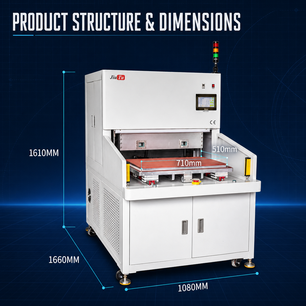
For the lamination stage, the 9TU-M040D Industrial Vacuum Laminating Machine is one model to examine when staged pressing and product-specific recipe settings are relevant. Its published configuration includes three automatic processing stages, with pressure, processing time and vacuum state configurable for each stage. The Siemens PLC and touchscreen support up to 14 stored recipes.
Single-Piece Lamination Evaluation
9TU-M040D Industrial Vacuum Laminating Machine
Its staged processing and recipe configuration can be relevant when evaluating different product settings. They do not establish a universal cycle time or guaranteed line output; those figures need to be measured with the intended panels, fixtures and operator workflow.
View machine details →Before accepting a throughput proposal, separate what the supplier measured from what was calculated or assumed. The quotation should state the tested product, loading quantity, cycle-time boundaries and operating conditions. If the target is reached only with maximum theoretical loads and no allowance for normal interruptions, the estimate still needs validation.
Frequently Asked Questions
Can rated cycle time predict daily output?
Not by itself. Rated cycle time does not necessarily include handling, batch loading, changeovers, downtime or quality losses. Estimate output from the complete station cycle and the actual bottleneck, then adjust for availability and first-pass yield.
How is mixed-model production estimated?
Weight each model’s station cycle by its expected share of total units, then add changeover time separately. For batch equipment, confirm that the products can share the same validated loading arrangement and process conditions.
When does adding a second station increase throughput?
When the existing station is the confirmed bottleneck and both stations can run independently in parallel. Shared operators, material supply or downstream capacity may limit the gain. Adding capacity at a station that already has spare capacity will not necessarily increase good output.
Production Capacity & Configuration Review
Check the Equipment Configuration Against Your Output Target
Before comparing machine models, establish what the line needs to deliver and what will pass through it. Include the details that determine cycle time, usable batch capacity and the likely bottleneck:
- Panel dimensions and LCD/OLED material stack
- Required good output and available shift time
- Expected product mix and changeover frequency
- Process sequence, fixtures and batch arrangement
With this information, an equipment discussion can focus on the operation that limits output and the trial data needed to validate the proposed configuration—rather than comparing nominal machine speeds in isolation.